Hydrogen bonding plays an important role in many chemical and biological processes, but this interaction is complex and has been difficult to quantify in correlation analysis. One of the better ways to describe hydrogen bonding strength is to use the thermodynamic parameters of H-bond formation: free energy (D G), enthalpy (D H), entropy (D S) and H-bond binding constant (K). These are connected to each other by the following relationships:

D G = - RTln K = D H - TD S (1)

It is possible to estimate the values of these parameters in the framework of a multiplicative approach based on equations (2) - (4) [1,2]:

D G = k'C_aC_d + k’_o (2)

D H = kE_aE_d (3)

log K = k"a b + k"_o (4)

where C_a and C_d are free energy H-bond acceptor and donor factors, E_a and E_d are enthalpy H-bond acceptor and donor factors, and a and b are H-bond donor and acceptor binding constants. Some limitations of this multiplicative approach inspired us to construct an overall H-bond acceptor scale on the basis of equation (5) [3]:

a C_ao =0.266a - logP (5)

The utility of eqs. (2) - (5) depends on the existence of vast, readily accessible experimental thermodynamic data, and a program to estimate thermodynamic parameters for new chemical compounds. HYBOT (Hydrogen Bond Thermodynamics), described in detail in ref. [2], is such a database and program.

On the basis of the previously noted factors, it is possible to construct QSAR descriptors for H-bonding. Table 1 summarizes information about such descriptors and identifies the computer programs that calculate and use those descriptors. These programs were created in the Department of Computer-Aided Molecular Design, Institute of Physiologically Active Compounds, Russian Academy of Sciences.

Table 1. Hydrogen bond descriptors and the programs used to generate them.

H-bonds are not the only interatomic interactions; therefore, the program HYBOT-PLUS was created to calculate descriptors for steric and electrostatic forces. In all, the program calculates 15 molecular descriptors: molecular polarizability (a ), maximal negative charge (q-_max), maximal positive charge (q+_max), sum of negative and positive charges ( a q- and a q+), C_amax, C_dmax, a C_a, a C_d, a C_ad, a q-/a , a q+/a , a C_a/a , a C_d/a and a C_ad/a . In addition it computes the polarizability, partial atomic charge and H-bond factor values for each atom in a molecule. The program uses the Structural Editor or MOL and SDF files for structural input, and Excel spreadsheets to report the results (Fig. 1).

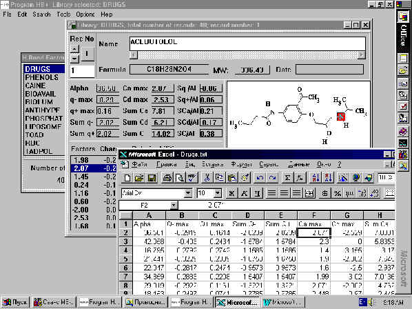
Fig 1. Results for acebutolol calculated by HYBOT-PLUS.

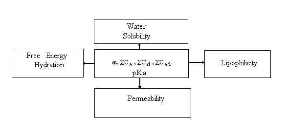
Fig. 2. Relationships between H-bond descriptors and chemical properties.

Free energy of hydration

D G_hyd = - 2.76(±0.80) - 5.12(±0.32)C_ad (6)

(n = 223, r = 0.903, s = 3.65, F = 977)

D G_hyd = - 1.05(±0.86) - 6.80(±0.55)C_a + 3.72 (±0.50)C_d (7)

( n= 223, R = 0.922, s = 3.29, F = 625)

D G_hyd = - 1.73(±1.45) - 0.072(±0.121)a - 6.89(±0.57)C_a + 3.62(±0.53)C_d (8)

(n = 223, R = 0.923, s = 3.29, F = 418)

Water solubility of liquid neutral compounds:

LogS_w = -0.258(±0.017)a + 1.08(±0.10)C_a - 0.20(±0.09)C_d ) (9)

(n = 142, R = 0.953, s = 0.38, F = 452)

Lipophilicity:

logP_oct-water = 0.266(± 0.030)a - 1.00(± 0.10)a C_a (10)

(n = 2850, R = 0.970, s = 0.23)

logP_ether/water = 0.303(± 0.077)a -1.42 (± 0.22) a C_a (11)

(n = 22, R = 0.928, s = 0.48, F = 123.1)

logP_{olive oil/water} = - 1.71(± 0.057) + 0.112(± 0.060)a - 0.30 (± 0.07)a C_ad (12)

(n = 22, R = 0.908, s = 0.65, F = 44.5)

D logP azole derivatives:

D logP_Oct-cyHex = - 0.76 (±1.53) + 0.22(±0.06)C_ad (13)

(n = 9, r = 0.951, s = 0.25, F = 66.4)

Alcohols and steroids:

D logP_Oct-Hep = 1.30(±0.40) + 0.17(±0.05)C_ad (14)

(n = 22, r = 0.834, s = 0.41, F = 45.6)

Human red cell basal permeability (BP) of alcohols, water, urea and thiourea [4]:

log BP = - 0.70(±0.64) + 1.08(±0.16)C_d (15)

(n = 10, r = 0.983, s = 0.43, r_cv = 0.976)

Permeation of non-electrolytes through cells of the alga Chara ceratophylla [4]:

log Per = 0.83(±0.57) + 0.59 (±0.12)C_d (16)

(n = 27, r = 0.903, s = 0.49, r_cv = 0.885)

Absorption and intraduodenal (id) bioavailability of azole endothelin antagonists [4]:

log AUC_id = -4.32(±1.05) + 0.41(±0.14)C_d (17)

(n = 9, r = 0.935, s = 0.32, r_cv = 0.818)

Human skin permeability coefficients (log k_p) of phenols [4]:

logk_p = - 8.72(±2.79) + 0.67(±0.15)C_d + 2.47(±1.28)logMW (18)

(n = 17, R = 0.949, s = 0.20, r_cv = 0.915)

Human skin permeability coefficients (log k_p) of alcohols and steroids :

logk_p = - 5.14(±0.45) - 0.47(±0.14)C_a + 0.23(±0.14)C_d + 0.038(±0.027)a (19)

(n = 22, R = 0.94, s = 0.42, r_cv = 0.914)

Caco-2 cell permeability of drugs [5] :

logk_p = - 4.10(±0.57) + 0.005(±0.002)logMW - 0.20(±0.03)C_ad (20)

(n = 17, R = 0.883)

Lecithin Siposomes permeability of phenols:

log k_p = 1.32(±0.51)+0.158(±0.032)a - 0.68(±0.14)C_a (21)

(n = 26, R = 0.939, s = 0.23, F = 85.4)

logk_p = 0.78(±0.79) + 0.171(±0.034)a - 0.69(±0.13)C_a-0.15(±0.13)C_d (22)

(n = 26, R = 0.947, s = 0.22, F = 63.3)

logk_p = 1.50(±0.72) + 0.173(±0.026)a - 0.75(±0.11)C_a - 0.15(±0.14)C_d

- 0.07(±0.04)pKa (23)

(n = 26, R = 0.970, s = 0.17, F = 82.6)

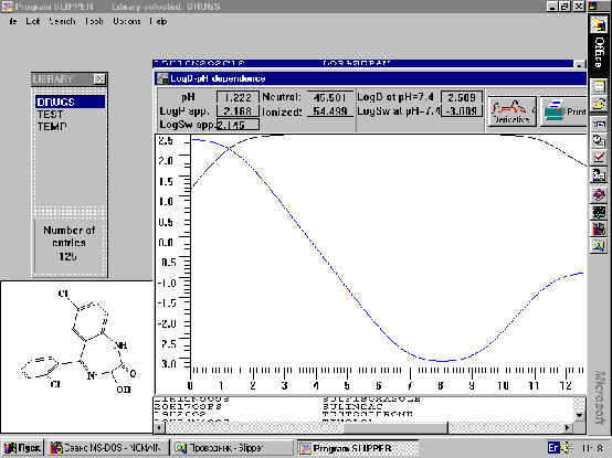
Fig.3. Lipophilicity and solubility pH dependent profiles generated by SLIPPER.

Because these new H-bond descriptors were successful in predicting lipophilicity and solubility, we were able to create the computer program SLIPPER (Solubility, LIPophilicity, PERmeability) [6]. The current version of the program calculates complete compound profiles of pKa-lipophilicity and pKa-water solubility on the basis of polarizability, H-bond factors and pKa.

An example of the results from such a calculation is presented in Fig. 3.

In addition, these H-bond descriptors can be useful in QSAR correlations of various biological activities. For example, there is the case of tadpole narcosis:

Log(1/C) = 0.98(± 0.22) + 0.221(± 0.018)a - 0.73(± 0.08)a Ca (24)

(n = 100, R = 0.932, s = 0.38, F = 323)

(1) Vitro fischeri.

Common narcotic models:

log1/EC₅₀ = 0.08(± 0.55) + 0.28(± 0.04)a (25)

(n = 48, r = 0.90, s = 0.44, F = 205)

log1/EC₅₀ = 0.50(± 0.54) + 0.27(± 0.04)a - 0.31(± 0.17)C_a (26)

(n = 48, R = 0.93, s = 0.39, F = 136)

Non-polar narcotic models:

log1/EC₅₀ = - 0.43(± 0.51) + 0.32(± 0.04)a (27)

(n = 33, r = 0.95, s = 0.37, F = 303)

log1/EC₅₀ = - 0.02(± 0.61) + 0.30(± 0.04)a - 0.27(± 0.24)C_a (28)

(n = 33, R = 0.96, s = 0.34, F = 175)

Polar narcotic models:

log1/EC₅₀ = 1.97(± 1.13) + 0.14(± 0.08)a (29)

(n = 15, r = 0.73, s = 0.38, F = 15)

log1/EC₅₀ = 2.80(± 0.93) + 0.14(± 0.06)a - 0.59(± 0.34)C_a (30)

(n = 15, R = 0.89, s = 0.26, F = 22)

(2) Daphnia magna.

Common narcotic models:

log1/EC₅₀ = 1.07(± 0.64) + 0.23(± 0.05)a (31)

(n = 35, r = 0.86, s = 0.34, F = 97)

log1/EC₅₀ = 1.46(± 0.61) + 0.22(± 0.042)a - 0.31(± 0.19)C_a (32)

(n = 35, R = 0.90, s = 0.30, F = 69)

Non-Polar narcotic models:

log1/EC₅₀ = 0.91(± 0.65) + 0.25(± 0.05)a (33)

(n = 23, r = 0.92, s = 0.30, F = 117)

log1/EC₅₀ = 1.36(± 0.84) + 0.23(± 0.05)a - 0.57(± 0.72)C_a (34)

(n = 23, R = 0.93, s = 0.29, F = 65)

Polar narcotic models:

log1/EC₅₀ = 5.33(± 0.58) - 1.01(± 0.038)C_a (35)

(n = 12, R = 0.88, s = 0.25, F = 36)

log1/EC₅₀ = 4.17(± 1.51) + 0.07(± 0.09)a - 0.87(± 0.38)C_a (36)

(n = 12, R = 0.92, s = 0.23, F = 24)

(3) Pimephales promelas.

Common narcotic models:

log1/EC₅₀ = - 0.38(± 0.79) + 0.32(± 0.06)a (37)

(n = 33, r = 0.90, s = 0.47, F = 129)

log1/EC₅₀ = 0.85(± 0.80) + 0.26(± 0.05)a - 0.51(± 0.22)C (38)

(n = 33, R = 0.94, s = 0.36, F = 120)

Non-Polar narcotic models:

log1/EC₅₀ = - 0.55(± 0.88) + 0.33(± 0.06)a (39)

(n = 23, r = 0.92, s = 0.48, F = 120)

log1/EC₅₀ = 1.07(± 0.72) + 0.25(± 0.05)a - 0.77(± 0.25)C_a (40)

(n = 23, R = 0.98, s = 0.30, F = 201)

Polar narcotic models:

log1/EC₅₀ = 5.08(± 0.69) - 0.87(± 0.44)C_a (41)

(n = 10, r = 0.85, s = 0.26, F = 21)

log1/EC₅₀ = 3.55(± 1.70) + 0.10(± 0.11)a - 0.76(± 0.38)C_a (42)

(n = 10, R = 0.92, s = 0.21, F = 19)

These new physico-chemical descriptors also can be used as estimates for similarity among chemicals and diversity in databases by yet another new computer program: MOLDIVS (MOLecular DIVersity and Similarity) [7].

To construct predictive QSAR models it is necessary to take the three dimensional properties of compounds into account. In 1987 Raevsky proposed that 3D structures could be described by the spectra of interatomic interactions [8]. In this approach each pair of atoms in a molecule gives a line in the spectrum for any type of interaction. A line’s position corresponds to the distance between the two atoms while its intensity corresponds to the product of physico-chemical parameters associated with those atoms. Atomic vibrations transform lines into bands; thus spectra of interatomic interactions are superpositions of all such bands. The computer programs MOLTRA (MOLecular Transform Analysis) and CONFAN (CONFormation Analysis) calculate the following interaction spectra: van-der-Waals, positive charges between each other, negative charges between each other, positive charges with negative ones, H-bond acceptors between each other, H-bond donors between each other and H-bond acceptors with H-bond donors. Examples of these spectra are presented on the left side of Fig.4. In principle, each point of such spectra can be used as a 3D descriptor. For example, in a QSAR study on the inhibition of phosphorylation of polyGAT by a -substituted benzylidenemalononitrile-5-S-aryltyrphostins, it was found that the interactions of two H-bond donors at the distance 7.4 A played an important role (eq. 43):

log 1/IC₅₀ = 0.64(±1.88) + 1.74(±0.10)LUMO + 0.39(±0.10)HB--7.4 (43)

(n = 12, R = 0.912, s = 0.37, F = 22.3)

log 1/K_i = 13.7 (±2.3) - 4.33(±1.43)logSIS++ (44)

(n = 15, r = 0.849, s = 0.50, F = 42.6)

log 1/K_i = 6.8 (±2.2)+ 0.092(±0.046)a -0.45(±0.19)a C_ad (45)

(n = 15, R = 0.910, s = 0.45, F = 28.9)

log 1/K_i = 14.6 (±4.1) + 0.076(±0.040)a - 6.06(±2.05)logSIS++ (46)

(n = 15, R = 0.940, s = 0.37, F = 45.5)

The right side of Fig. 4 shows molecular H-bond potentials for two compounds; Goodford’s approach was used [9]. However, here we used enthalpy H-bond factor values (eq. 3) of concrete atoms of two molecules which are interacting between each other.

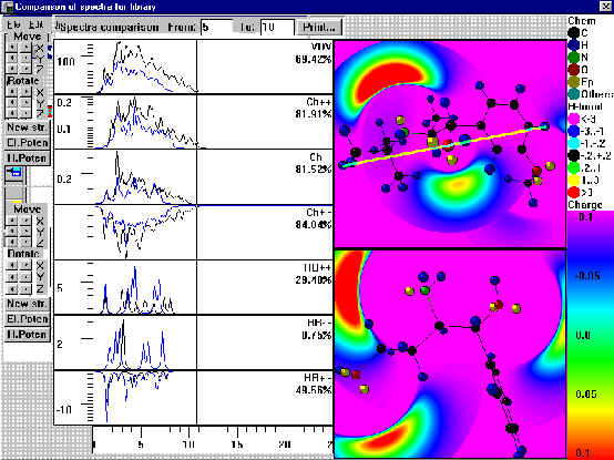
Fig.4. Spectra of interatomic interactions, Similarity Indexes of Spectra of interatomic interactions and H-bond potentials for any pair of compounds.

In summary, we have developed a method for the quantitative description of H-bonding that is founded on large databases of thermodynamic parameters and H-bond factors (the program HYBOT). Supplementing this are other programs. HYBOT-PLUS calculates H-bond descriptors, polarizabilities and partial atomic charges. SLIPPER estimates important properties as water solubility and the lipophilicity-pKa profile. Based on structural fragments, MOLDIVS affords a measure for similarities and diversities among a set of compounds. MOLTRA calculates 3D H-bond descriptors. CONFAN estimates similarities among H-bond donors and acceptors. These programs afford new and quantitative descriptors for H-bonding. Combined with two other important terms for interatomic interactions (steric and electrostatic forces) they can be used broadly in Drug Design and QSAR.

REFERENCES:

1. O.A. Raevsky, J.Phys.Org.Chem., 10, 404-412 (1997).
2. O.A. Raevsky, in Computer-Assisted Lead Finding and Optimization, eds.H. van de Waterbeemd, B. Testa, G. Folkers, 1997, Basel: Wiley-VHC, pp. 367-378.
3. O.A. Raevsky, V.Ju. Grigor'ev, Chim.-Farm.z. (Rus.), 1998, in press.
4. O.A. Raevsky, K.-J. Schaper, Eur.J.Med.Chem., v. (1998), in press
5. H. van de Waterbeemd, G .Gamenisch, G. Folkers, O.A. Raevsky, Quant.Struct.-Act.Relat, 15, 480-490 (1996);
6. O.A. Raevsky, S.V. Trepalin, L.P. Trepalina, this volume,
7. V.A. Gerasimenko, S.V. Trepalin, O.A. Raevsky, this volume,
8. O.A Raevsky, in QSAR in Drug Design and Toxicology, eds. D. Hadzy, B. Jerman-Blazic, 1987, Amsterdam: Elsevier, pp. 31-36.
9. R.C. Wade, K.J. Clark, P.J. Goodford, J.Med.Chem., 36, p.148 (1993).